How to Run Monte Carlo Simulations in Excel (Updated Aug 2024)
So you want to run Monte Carlo simulations in Excel, but your project isn’t large enough or you don’t do this type of probabilistic analysis enough to warrant buying an expensive add-in. Well, you’ve come to the right place. Excel’s built-in functionality allows for stochastic modeling, including running as many simulations as your computer’s processing power will support, and this short post with video tutorial walks you through the setup and the process of running Monte Carlo simulations in Excel without any add-ins necessary.
Probabilistic Analysis from a Real Estate Perspective
This is a commercial real estate blog, and therefore this tutorial looks at stochastic modeling from the perspective of a real estate professional. However, the great majority of the techniques shown in this post will work across disciplines.
I’ll also note, several of the concepts shown here I adapted from Keith Chin-Kee Leung’s excellente graduate thesis on the subject: Beyond DCF Analysis in Real Estate Financial Modeling: Probabilistic Evaluation of Real Estate Ventures.

Monte Carlo Simulations for Real Estate – Excel Nerd Level: 1,000,000
What This Tutorial is Not
This post is not a course on probability analysis. As such, it assumes you have a basic understanding of probability, statistics, Excel, and know what a Monte Carlo simulation is. If you’d like to get a refresher on probability or statistics in general, I recommend taking a course on the subject. Here’s a free MOOC (massive open online course) offered by Duke:
The Scenario – An Apartment Deal
Before running your simulations, you’ll need a scenario to model. In this case, we’re going to run a basic discounted cash flow on a hypothetical apartment building to determine how much we’d be willing to pay for the property today. Here is what we know:
- The subject property has 10 units
- The subject property charges $1000/month for each unit; rents grow by 3% last year
- There is one unit vacant, and for simplicity we assume there will always be one unit vacant
- Expenses are $3,000 per month; expenses grow by 2% last year
- Comparable properties sell for a 5.5% – 6.0% cap rate today, but cap rates are expected to grow by about 5 basis points per year in the coming years (exit cap rate between 5.75% and 6.25%)
- Plan to hold the property for five years
- Target an 8% unleveraged return
Setting Up the Model
Next, I set up my Excel model in preparation for running the simulations (you can download the Excel workbook used in this tutorial at the end of this post).
- In column B and D, I drop in my base assumptions
- Cell G2 I label “DCF Value”
- In row 14, starting in cell F14 through K14, I add a period header with six periods including a period zero
- Cell E15 I label “Rent”
- Cell E16 I label “Expense”
- Cell E17 I label “Net Operating Income”
- Cell E18 I label “Residual Value”
- Cell L17 I label “Exit Cap”
- Cell E19 I lable “Net Cash Flow”
- Cell D14 I label “Growth Rate”
- In Cell G15 I write the formula: =9*12*$D$4*(1+$D15)^(G14-1) which means nine units (10 units less one vacant unit), times 12 months, times $D$4 ($1000 rent/unit/month), times one plus $D15 (the probable growth rate calculated in cell D15), raised to the period (G15) minus one (I subtract one because we don’t want rent to grow in year one). Since the proper absolute cell references have been created (e.g. $D$4 and $D15), I can then copy the formula right to cell K15.
- I follow a similar process for expenses, using the formula: =$D$7*12*(1+$D16)^(G14-1) in cell G16 and then copying that formula out to cell K16.
- In cells G17 through K17, I subtract expenses from rent (e.g. in G17 I write =G15-G16) to arrive at a net operating income for each year.
- In cell K18 I write the formula: =K17/L18 which means divide year five net operating income by the probable exit cap rate (L18).
- In cells G19 through K19 I add up the net cash flows for each year: net operating income in years one through four and net operating income plus residual value in year five.
- Finally, in cell G3 I calculate the present value of the cash flow stream in row 19 discounted back at 8% (the target unleveraged return) using the formula: =NPV(D12,G19:K19).
With the DCF set up, I can now move on to adding probability to my assumptions.

Adding Probability using the RANDBETWEEN() Function
In our scenario above, we have a couple of assumptions that are uncertain, and therefore would be great candidates for adding variability to. First, we need to choose a distribution type for our probability.
We have a number of options, the two most common being uniform distribution (constant probability where all outcomes are equally likely) and normal distribution (think bell curve probability where the resulting value is likely to be closer to the mean). For simplicity’s sake, we will choose a uniform distribution.
- In cell D15, I add uniform variability to the rent growth rate using the formula: =$D$5*RANDBETWEEN(-500,2000)/1000, which means take 3% (last year’s rent growth from cell $D$5) and multiple it by a random number between -0.5 and 2.0 (RANDBETWEEN(-50,200)/100) so that the resulting rent growth rate falls randomly between -1.5% and 6.0%.
- In cell D16, I add uniform variability to the expense growth rate using a similar formula: =$D$8*RANDBETWEEN(-500,2000)/1000, only in this case I take last year’s expense growth rate (2% from cell $D$8) and multiply it by a random number between -0.5 and 2.0 (RANDBETWEEN(-50,200)/100) so that the resulting expense growth rate falls randomly between -1.0% and 4.0%.
- Finally, in Cell L18, I add uniform variability to the exit cap rate using the formula: =D10*RANDBETWEEN(958.3,1041.7)/1000, which means take 6% (the average between the 5.75% and 6.25% expected range for exit cap rates in year five) and multiple it by a random number between 0.9583 and 1.0417 (RANDBETWEEN(958.3,1041.7)/1000) so that the resulting exit cap rate falls randomly between 5.75% and 6.25%.
You will see now when you press F9, that the rent growth rate, expense growth rate, and exit cap rate values change randomly, resulting in a random change in the cash flows and the overall discounted cash flow value.
Running Monte Carlo Simulations using Data Tables
With probability added to your model, you can begin to run your Monte Carlo simulations. This process involves building a data table, linked to your DCF value (G3) so that each simulation records the resulting DCF value from that simulation.
Here is how we run the Monte Carlo Simulations using the Data Table feature in Excel:
- Cell B27 I label “Simulation #”
- I link Cell C27 to the DCF Value (=G3)
- I number cells B28 through B1027 from 1 to 1000. To do this, I first set cell B28 to 1. I next enter the formula =B28+1 into cell B29. Lastly, I copy the formula in B29 down to cell B1027.
- With the simulations numbered and cell C27 linked to the DCF value, I select cells B27 through C1027 and click the ‘Data table’ feature (Data>What-If-Analysis>Data Table).
- I leave the ‘Row input cell:’ box blank, and click on the ‘Column input cell’ box. I select an empty cell in the worksheet (which cell does not matter so long as it is a cell that is always blank), hit enter, and then ‘OK’.
- The data table will update with 1,000 iterations of our simulation and voila you’ve run a Monte Carlo simulation in Excel using the data table.
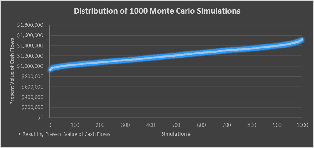
The probable range of values, with $1.2 million being the “Expected Value”
The Expected Value – What You Might be Willing to Pay
The mean (average) of all the simulations is your “Expected Value” or what you might be willing to pay for the subject property given your assumptions. In my case, the expected value is about $1.2 million.
I also like to calculate the minimum, maximum, and standard deviation of the simulations to get a feel for the range of the values. So for instance, in this case, the minimum is around $925,000 and the maximum is around $1.5 million. What this means is that there was an instance where I would need to pay $925,000 in order to hit an 8% return and there was an instance where I could pay $1.5 million to hit an 8% return.
Nonetheless, the more simulations you run, the more the values will create a normative pattern where you have a 68% probability that the value will be one standard deviation from the mean and a 95% probability that the value will be two standard deviations from the mean (the 68-95-99 rule). Therefore, the smaller the standard deviation, the more certain you can be about your expected value.
So in conclusion, for our hypothetical apartment building, we’d be willing to pay somewhere between $925,000 and $1.5 million with $1.2 million being the most likely purchase price.
Video Tutorial – Running Monte Carlo Simulations in Real Estate
As a complement to the written tutorial above, I’ve recorded a video that walks through doing your own Monte Carlo simulations for real estate in Excel.
Follow Along Using the Excel File from the Video
To make this Monte Carlo simulation tutorial accessible to everyone, it is offered on a “Pay What You’re Able” basis with no minimum (enter $0 if you’d like) or maximum (your support helps keep the content coming – similar real estate course modules sell for $100 – $300+). Just enter a price together with an email address to send the download link to, and then click ‘Continue’. If you have any questions about our “Pay What You’re Able” program or why we offer our models on this basis, please reach out to either Mike or Spencer.
Conclusion
In conclusion, by leveraging Excel’s built-in functionality, you can effectively run Monte Carlo simulations without the need for costly add-ins. To continue expanding your knowledge of Monte Carlo Simulations and other commercial real estate concepts, consider checking out our A.CRE AI Assistant. This tool uses AI to provide personalized guidance, answer your CRE questions, and help you with financial modeling and analysis. Whether you’re a seasoned professional or new to the field, the A.CRE AI Assistant can enhance your understanding and efficiency.


