When Prices Stopped Rising: 2008 Crisis, Part 5

Part 5 of my series working through the 2008 financial crisis from a real estate perspective, and the part where the assumption everything rested on finally gets tested. If you’re new to the series, in Part 1 I looked at why the mortgage was trusted, in Part 2 I followed a single mortgage payment down the chain and watched the risk detach from everyone who touched it, in Part 3 I opened up the tower of tranches and CDOs, and in Part 4 I showed how the bets on that tower outgrew the mortgage market itself. Here I want to look at what was actually happening inside the loans while all of that was being built, and at the mechanism that made every one of them fail at the same moment.

Every part of this series so far has ended by pointing at the same load-bearing assumption. The tranches in Part 3 needed losses to stay inside a thin band. The correlation input needed defaults to be independent. The protection AIG wrote in Part 4 needed spreads to stay calm. All of it rested on the belief that American mortgages would not deteriorate all at once.

This part is about why they were always going to.

The Credit Cycle You Have Already Watched From the Inside

If you have underwritten commercial real estate through a full cycle, you already know how standards erode, because you have watched it happen in slow motion.

It never arrives as a decision. Nobody circulates a memo announcing that the shop is lowering its bar. What happens is drift. The debt service coverage floor slides from 1.30 to 1.25, then to 1.20 because a competitor is quoting it. Loan to value creeps. Pro forma rents start showing up where in-place rents used to be. Interest-only periods stretch from one year to two to the full term. Each concession is defensible on its own deal, and every one of them is made by someone who can explain exactly why this borrower and this asset are the exception.

The erosion is only visible if you look at the portfolio in aggregate over time, and by then you have already written the loans.

That is the story of subprime origination between 2004 and 2006, with one difference that turns out to matter enormously. In commercial real estate, the loan is underwritten against an asset that produces income. In subprime, the loan was increasingly underwritten against an asset that produced nothing except price appreciation.

The Averages Held While the Pool Changed Underneath Them

Here is the detail I keep returning to, because it is the third time this series has run into the same failure and the first time we can watch it happening in real time.

Michael Burry was reading loan prospectuses. Not summaries, the actual documents, which were public and cost about a hundred dollars a year to access and which almost nobody outside the drafting lawyers bothered to open. Because subprime lenders issued bonds sequentially, each one containing loans originated in a particular window, you could line the prospectuses up and watch the product change quarter by quarter.

What he found, in Lewis’s account, is the whole story of Part 5 in a single data series. Two-year fixed, twenty-eight year floating interest-only ARMs were 5.85 percent of the pool in early 2004. By late 2004 they were 17.48 percent. By late summer 2005 they were 25.34 percent.

And over that same stretch, the average FICO score of the pool, the share of no-documentation loans, and the loan-to-value measures all stayed roughly static.

Sit with what that means. The pool got dramatically more fragile while every headline statistic describing it stayed flat. A rating model reading pool averages would have registered no change at all. Not a small change. None.

This is not just one investor’s reading of the prospectuses. Yuliya Demyanyk and Otto Van Hemert later ran the loan-level data covering the large majority of securitized subprime, adjusting loan performance for borrower characteristics, loan characteristics, and subsequent house price appreciation. They found that loan quality deteriorated for six consecutive years before the crisis, monotonically, and that securitizers were to some extent aware of it. Their conclusion is the thesis of this entire part in one line: the problems could have been detected long before the crisis, but they were masked by high house price appreciation between 2003 and 2005.

It is worth noting what the deterioration was not confined to. It showed up across hybrids and fixed-rate loans, purchase and cash-out, low-documentation and full-documentation alike. This was not one bad product. It was the whole cohort.

The Bottom Had a Name

In Burry’s reading, by 2005 standards had not merely fallen. They had hit bottom, and the bottom was a specific product: the interest-only negative-amortizing adjustable-rate subprime mortgage.

Read that string of adjectives slowly, because each one removes a piece of what makes a loan a loan. Adjustable rate means the payment is not fixed. Interest-only means no principal is being repaid. Negative amortizing means the borrower can pay less than the interest due, with the shortfall added to the balance.

Put together, they describe an arrangement in which the borrower can pay nothing at all and watch the amount owed grow. That is not credit extended against income. It is a position in the price of the house, with the lender holding the other side.

A Thirty-Year Loan Built to Last Two

The mechanism that made this work, for as long as it worked, was the teaser rate.

Subprime loans of this era were typically fixed for two or three years at an artificially low rate, then reset to a much higher floating “go-to” rate. Steve Eisman’s description of the logic, in Lewis’s account, is that lenders were making loans at the teaser rate to people they knew could not afford the go-to rate, specifically so that those borrowers would be forced to refinance, which is where the lender made more money.

The thirty-year term was cosmetic. These were two-year loans with a thirty-year label, and the exit was always a refinance.

Any commercial real estate professional should feel something click here. That is a bridge loan. Short fixed period, payment that jumps at the reset, repayment dependent not on the borrower’s cash flow but on a takeout at the end. We underwrite these constantly, and the entire discipline of underwriting one comes down to a single question: is the exit real?

For a bridge loan on a building, the exit is a stabilized asset that a permanent lender will finance, and you test it by underwriting the stabilized cash flow. For these mortgages, the exit was a refinance, a refinance requires equity, and the borrower had put in almost none. So where was the equity supposed to come from?

Appreciation. Only appreciation. That was the entire underwriting.

What Actually Breaks Is the Exit

This is where the arithmetic becomes unforgiving.

Write down the equity a borrower has available at the moment of refinance. Approximately:

E = (1 – LTV) + g x t + a

Take the terms one at a time. LTV is the loan-to-value at origination, so (1 – LTV) is whatever equity the borrower started with. g is annual house price appreciation and t is years elapsed, so g x t is the equity that appreciation delivers over the teaser period. a is cumulative amortization, the equity the borrower builds by paying down principal.

Now put in the actual values from this market. LTV was frequently at or near 100 percent, sometimes above it once a silent second was stacked behind the first, so the first term is approximately zero. Amortization is normally positive and helps you, but under an interest-only loan it is exactly zero, and under negative amortization it is negative. The balance grows.

Which leaves g x t carrying the entire structure. Every dollar of equity that borrower needs in order to refinance has to come from appreciation, because the other two terms contribute nothing or worse.

So set g to zero and see what happens. Not negative. Zero. Prices merely stop rising.

The first term is still zero. Amortization is still zero or negative. And g x t is now zero. The borrower arrives at the reset date with no equity, facing a payment that has just jumped to the go-to rate, and there is no refinance available at any price, because there is nothing to refinance against.

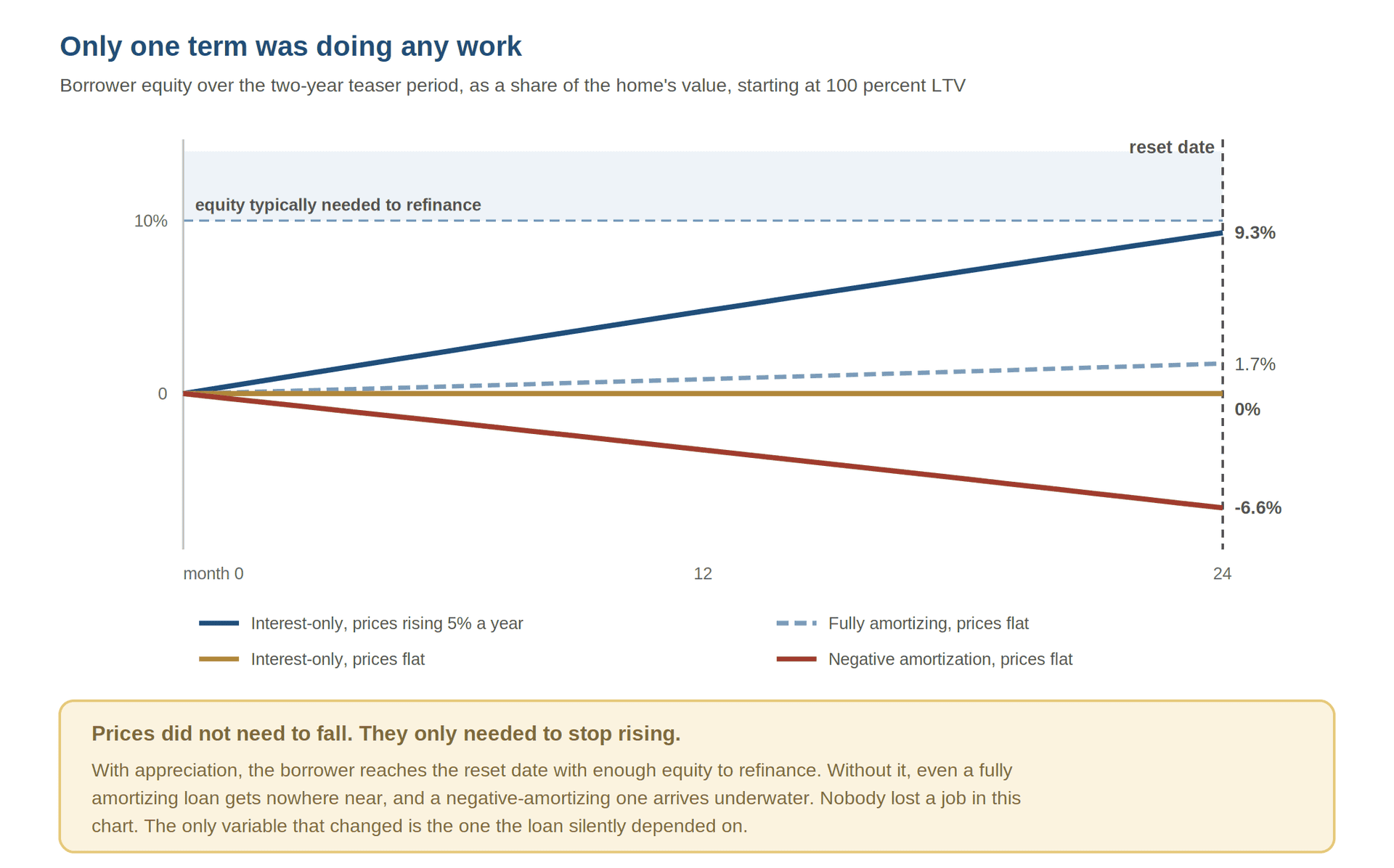
Nothing about the borrower changed. They did not lose a job. The economy did not contract. The only thing that changed is that the appreciation the loan silently required stopped showing up.

Lewis puts the consequence plainly: house prices did not need to fall for enormous numbers of Americans to default. They only needed to stop rising at the extraordinary rates of the preceding years.

The Rating Agencies Knew This, and Said So Out Loud

Here is the part I did not expect to find, and it is the most damning document I came across while working on this piece.

In March 2007, Robert Rodriguez of First Pacific Advisors was on a call with Fitch about the subprime securitization market. Fitch, by his account, was confident in its models. His colleague asked what the key drivers of the rating model actually were. Fitch answered: FICO scores, and home price appreciation in the low to mid single digits, as it had been for the past fifty years.

So they asked the obvious follow-up. What if appreciation went flat for an extended period? The model would start to break down. What if prices declined one or two percent for an extended period? Fitch’s answer was that the models would break down “completely.” And how far up the rating scale would a two percent decline reach? As high as the AA or AAA tranches.

That exchange took place roughly six months before the collapse, with a rating agency describing its own model. The dependency was not hidden and it was not a subtle artifact that only became visible in hindsight. It was the acknowledged, primary input.

I find that clarifying in a way the usual account of the crisis is not. Nobody needed to discover this later. Somebody asked, and got a straight answer.

Why the Correlation Was Always One

Now we can close the loop that Part 3 opened and Part 4 carried.

In Part 3, the rating agencies modeled the correlation between subprime tranches at around 30 percent, and the entire investment-grade rating of a CDO depended on that number being small. In Part 4 we saw that the Gaussian copula compressed the dependence among thousands of loans into a single correlation parameter. I said at the time that the real correlation was close to one. Here is the precise reason.

A single-factor model says that each exposure’s outcome is driven partly by a common factor and partly by something idiosyncratic to itself:

Loss = β x F + ε

F is the common factor affecting everyone, β is how strongly a given exposure depends on it, and ε is that exposure’s own individual circumstances. In that setup the correlation between any two exposures works out to approximately:

ρ ≈ β²

Diversification lives entirely in ε. If borrowers default for reasons particular to themselves, a job loss here, a divorce there, an illness somewhere else, then β is small, the idiosyncratic terms dominate, and pooling genuinely works. That is the world the models assumed.

But we just established what these loans actually depended on. Not the borrower’s income. Not the borrower’s circumstances. House price appreciation, and nothing else, for essentially every loan written this way. So F was house price appreciation, β was close to one, and therefore ρ was close to one. Not because the loans were geographically concentrated, but because the product had been engineered so that every loan hung from the same hook.

It is worth seeing what that does to the shape of the outcome, because this is the piece that makes the tranche math work or fail. The standard result, from Oldrich Vasicek, gives the fraction of a large pool that defaults once you know how the common factor turned out:

Default rate = N[ ( N⁻¹(p) – √ρ x Y ) ÷ √(1 – ρ) ]

Take the terms one at a time. p is the average default probability across the pool. Y is the realized value of the common factor, the economy, and in our case house prices. N is the cumulative normal distribution and N⁻¹ is its inverse, which is just the machinery that converts probabilities into standardized units and back. ρ is the correlation.

What matters is not the notation but what the expression does as you turn ρ. When ρ is near zero, the √ρ term vanishes, Y drops out, and the pool defaults at roughly its average rate no matter what the economy does. Outcomes cluster tightly around the mean, which is exactly the behavior a senior tranche needs.

As ρ rises toward one, Y starts to dominate. The realized default rate stops tracking the average and starts tracking the factor. Good draw of Y and almost nothing defaults. Bad draw and almost everything does. The average is unchanged. The distribution has gone from a cluster to a barbell.

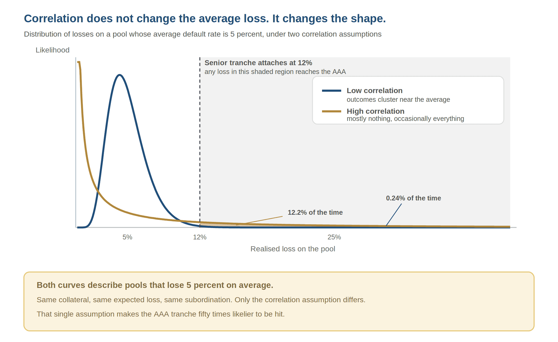
That is the whole thing, in one line of algebra. Correlation does not change how much you expect to lose. It changes the shape of the loss distribution, and a tranche is nothing but a claim on a slice of that shape.

Joshua Coval, Jakub Jurek and Erik Stafford worked out the consequence, and the arithmetic is simple enough to do in your head. Take two bonds, each with a 10 percent chance of default, and tranche them. If the defaults are uncorrelated, the senior claim defaults only 1 percent of the time. If they are perfectly correlated, the senior claim inherits the full 10 percent of the underlying. Same bonds, same structure, same subordination. One assumption, and the senior tranche becomes ten times riskier.

Their simulation of a full CDO makes the same point on the rating scale. Holding everything else fixed and moving only the correlation, a senior tranche rated AAA at a correlation of 20 percent falls to BBB– at 60 percent, and to BB at 80 percent. And when the structure is a CDO built from the mezzanine tranches of other CDOs, which is what most subprime CDOs actually were, that same shift wipes out a quarter of the value of a claim that was investment grade under the baseline.

Their conclusion is the sentence I would put above the desk of anyone rating structured credit: small errors that would be immaterial in the single-name market are significantly magnified by tranching, and magnified again when CDOs are built from other CDOs.

The Financial Crisis Inquiry Commission later documented how far the assumption had drifted. Moody’s had estimated that two mortgage-backed securities were less closely correlated than two securities backed by credit card or auto loans. In December 2008, it discarded its key CDO assumptions and replaced them with asset correlations roughly two to three times higher than what it had used before the crisis.

The Turn, in Order

The sequence is worth laying out, because it took longer than people remember.

Through the second half of 2005, the monthly remittance reports still looked fine. Credit quality was holding.

In June 2006, national home prices began to fall for the first time.

Then eighteen months of almost nothing. Between mid-2005 and early 2007 there was a widening disconnect between what subprime mortgage bonds were priced at and what the underlying loans were actually worth, and the market simply did not close it.

On January 31, 2007, the ABX, the publicly traded index of triple-B subprime bonds, fell from 93.03 to 91.98. A single point. That was the crack.

On April 2, 2007, New Century, the largest subprime lender in the country, was overwhelmed by defaults and filed for bankruptcy.

And in June 2007, investors in the collapsed Bear Stearns hedge funds were told that their $1.6 billion of triple-A rated subprime-backed CDOs had not lost some value. They were worthless.

That last sentence is the one I would ask you to hold onto. Not impaired. Not marked down. Worthless, at the top of the capital structure, in the tranche whose entire claim to safety was that everything beneath it would absorb the losses first.

Where the Story Goes Next

The assumption failed exactly as the structure required it to fail. The losses did not trickle in. They arrived everywhere at once, because everything was hanging from the same hook, and the subordination protecting the senior claims had been sized for a world in which that could not happen.

But large losses do not, by themselves, stop a financial system. Institutions fail and get absorbed. What happened next was something else, and it comes straight out of Part 4.

When Lehman Brothers failed, the market had to work out what the credit default swaps written against it were worth. The gross notional referencing Lehman was estimated at around $400 billion. With the recovery set by auction at 8.625 cents on the dollar, that implied protection sellers owing buyers something on the order of $366 billion.

The actual net settlement, once offsetting positions were compressed against each other, came to roughly $6 billion.

Both numbers describe the same contracts. And for the critical weeks, nobody could tell you which one was real, because these were private bilateral agreements with no central record of who had written what to whom.

For now, what I’m taking away from this part is that the question which froze the system was never how much money had been lost. It was whether the institution on the other side of your hedge was still standing, and there was no way to find out.

That is Part 6.

Sources and Further Reading

This series is built on two narrative accounts of the crisis, supplemented by the academic and official record. If you want the full story, go to the originals:

Lewis, Michael. The Big Short: Inside the Doomsday Machine. W. W. Norton, 2010.

Sorkin, Andrew Ross. Too Big to Fail. Viking, 2009.

Coval, Joshua, Jakub Jurek, and Erik Stafford. “The Economics of Structured Finance.” Journal of Economic Perspectives 23, no. 1 (2009): 3-25.

Demyanyk, Yuliya, and Otto Van Hemert. “Understanding the Subprime Mortgage Crisis.” Review of Financial Studies 24, no. 6 (2011): 1848-1880.

Vasicek, Oldrich. “The Distribution of Loan Portfolio Value.” Risk 15, no. 12 (2002): 160-162.

Financial Crisis Inquiry Commission. The Financial Crisis Inquiry Report. U.S. Government Printing Office, 2011.

---

Frequently Asked Questions about Subprime Mortgage Standards and the 2008 Financial Crisis

---