Linear Mortgage Payment Schedule Tool (Updated July 2024)
We recently shared a new modeling test to our library of real estate case studies entitled UK Debt Advisory Firm Modeling Test. In that case study, the test asked the real estate professional to analyze the returns of three different debt options. Two of those debt options include a type of mortgage called a linear mortgage, wherein the loan amortizes on a straight-line (i.e. principal payments are the same each period) rather than by the more common annuity method.
After completing the solution to that modeling test, I thought it would be worthwhile to build and share a module for calculating the payment schedule of a linear mortgage. In this post, I share that module with the A.CRE audience. I also share a short video tutorial on how to use the module.
Are you an Accelerator member? The UK Debt Advisory Firm Modeling Test was initially shared by an Accelerator member in the UK. Consequently, Accelerator members can download the solution to all case studies (and view video explanations when available) free by clicking here.
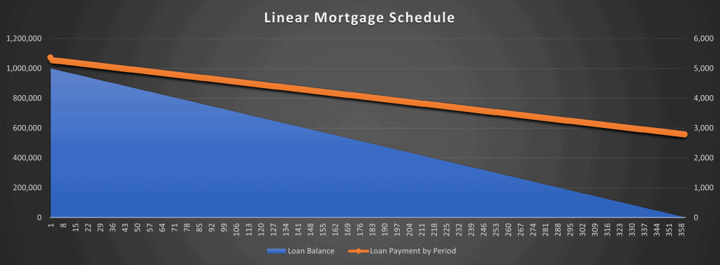
The loan balance decreases in a linear (i.e. straight-line) fashion with a linear mortgage.
What is a Linear Mortgage (vs. an Annuity Mortgage)?
Before talking through how to use this module, let’s first look at what a linear mortgage is. A linear mortgage is a mortgage wherein the principal amount due in each period is static. The result is that the loan balance decreases in a linear fashion (see visual above).
This is in contrast to the annuity mortgage, the most common type of mortgage in the United States, where the payment remains static and the amount of principal paid increases over time as the loan balance decreases (see visual below).
Until today, every model in the A.CRE Library of Real Estate Excel Models used a annuity-style mortgage. But given our global audience, and the prominence of the linear mortgage in markets such as the UK, I thought I’d share this module.
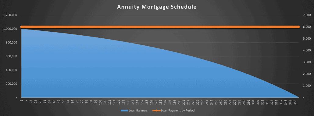
The loan balance decreases in a logrithmic fashion, while the loan payment is static.
What’s Included in the Linear Mortgage Payment Schedule Module
This module is fairly straightforward, but includes a few advanced features to provide a fair amount of flexibility. Here are a few of the features/elements of this module:
- Fixed interest rate. The module assumes a fixed interest rate. With that said, I’ve broken out the periodic interest in column L. This allows the user to easily replace the fixed rate with a variable rate.
- 30/360, Actual/360, and Actual/365 interest calculation. The module allows you to choose among three common interest calculation methods.
- Amortization per annum. The principal paid in each period is a function of the ‘amortization per annum’ input. This is a variation on the ‘amortization period’ input in our other amortization schedule modules, wherein the input determines how many periods it will take to pay the loan off. If 50% is entered for amortization per annum, the loan would be paid off in two years (1/50%). If 3.3333% is entered for amortization per annum, the loan would be paid off in 30 years (1/3.3333%).
- Dynamic loan term. The module allows for a loan term that is less than the period required to fully pay the loan off. This results in a balloon balance that is paid at maturity. So if the amortization per annum is 3.33333% (i.e. 30 years), and the loan term is 120 months, than a balloon balance equal to 66.6667% will be due at the end of year 10.
- Lender Yield. The model calculates lender yield (i.e. APR). If no lender fees are included (i.e. cell F6), than the lender yield will be equal to the fixed interest. However, with the lender fees input you can see what the lender yield is compared to the fixed rate to better understand the actual cost of the mortgage.
How to Use the Linear Mortgage Payment Schedule
Now using the module is quite simple. Drag and drop the worksheet from the module file into your own model, enter the inputs consistent with your situation, and than link the module cash flows to your own model.
Here are the inputs you’ll need to enter:
- Loan funding date. This is the date the loan closes, and will likely be equal to your analysis start date.
- Loan amount. This is the initial loan amount, before any lender fees.
- Lender fees. The fees charged by the lender to originate the loan. These only include the fees collected by the lender, and should not include other closing costs associated with the mortgage.
- Interest rate. The fixed annual interest rate quoted by the lender.
- Interest calculation method. The method by which the lender will calculate interest. The 30/360 method assumes a 30 day month, and 360 day year. The Actual/360 method assumes the actual number of days per month, with a 360 day year. And the Actual/365 method assumes the actual number of days per month, with a 365 day year.
- Amortization per annum. This is the percentage of the loan amount that amortizes (i.e. is paid down) each year. So if the initial loan amount is 100,000, and the amortization per annum is 5%, than 5,000 in principal will be due each year.
- Loan term. This is the number of months that the loan will be outstanding. The loan term is equal to or less than the number of periods required to pay the loan off. So if the amortization per annum results in a loan paid off in 240 months (i.e. 20 years), and the loan term is 10 years, than there will be a loan balance equal to 50% of the initial loan amount due as a balloon payment at the end of year 10.
Video Walkthrough of the Linear Mortgage Payment Schedule
As a supplement to the module, and the written instruction above, here is a video walkthrough of the linear mortgage payment schedule module:
ADDITIONAL RESOURCES
As an additional resource to modeling debt, we recommend using our Advanced Amortization Table Creator GPT. This tool allows for more sophisticated tracking and analysis of debt payments and amortization schedules. This tool offers customized schedules for various loan structures, flexible inputs of different loan terms, interest rates, and payment frequencies, and a schedule you can automatically updated based on changes in loan assumptions or refinancing terms. By leveraging the advanced features of this tool, you can create more robust and accurate financial models, streamlining the debt modeling process and gaining deeper insights into your real estate financing strategies.
In addition, you can find our Excel tool for modeling debt here.
Download the Linear Mortgage Payment Schedule
To make this model accessible to everyone, it is offered on a “Pay What You’re Able” basis with no minimum (enter $0 if you’d like) or maximum (your support helps keep the content coming – typical real estate Excel modules sell for $100 – $300+ per license). Just enter a price together with an email address to send the download link to, and then click ‘Continue’. If you have any questions about our “Pay What You’re Able” program or why we offer our models on this basis, please reach out to either Michael or Spencer.
We regularly update the model (see version notes). Paid contributors to the model receive a new download link via email each time the model is updated.
Frequently Asked Questions about the Linear Mortgage Payment Schedule Tool
Version Notes
v1.1
- Fixed issue where interest wasn’t calculating correctly in period 1
- Increased potential loan term to 40 years
- Added ‘Annual Cash Flow’ section
- Added line chart to visualize remaining loan balance by year
- Added titles to Monthly Cash Flow and Annual Cash Flow sections
- Updated placeholder values
- Misc. formatting updates
v1.0
- Initial release

