Watch Me Build Data Tables For Real Estate Sensitivity Analysis
This is a 3 part mini-series on using data tables in Excel to perform real estate sensitivity analysis. In this series, I’ll walk you through how to build both one-variable and two-variable data tables in parts 1 and 2. And in Part 3, I’ll walk you through how to no longer limit your two-variable sensitivity analysis to the impacts on only one dependent variable, but on an unlimited amount of dependent variables simultaneously.
To download all the templates for this mini-series, please click here or scroll down to the bottom of this post.
Are you an Accelerator Advanced member? Check out course 4, lesson 2 of the ‘Advanced Modeling – Property and Portfolio’ endorsement for additional techniques for performing real estate sensitivity analysis. Not yet an Accelerator member? Consider joining the real estate financial modeling training program used by top real estate companies and elite universities to train the next generation of CRE professionals.
Note: This series was previously split into three separate posts, but for the purposes of making this easier to navigate, I’ve aggregated them all into one place and reworked the text a bit.

Excel’s data table feature is one of the most effective ways to perform scenario analysis in real estate financial modeling.
Creating Data Tables Part 1: One Variable Data Table
This first section is actually an update and addition to one of my first posts on A.CRE, ‘How to Build a One Variable Data Table’.
I actually haven’t thought much about that post since I published it back in 2015, but recently I had a question come in asking how to solve for simultaneously showing what happens to return metrics as you change the purchase price of a model. This person wanted to know if there was a solution to this outside of manually changing the purchase price and then copying and pasting the results for each new price he entered.
What he was asking for was a one variable sensitivity analysis using excel’s data table function. So remembering that I wrote this post years back, I looked it up to share it with him and when I reviewed it I realized how, for lack of a better word, primitive, it looked.
So as a result, I decided to update the post with a second example using a video and downloadable template for you to follow along. Now for nostalgic purposes and also to provide you with a second example, I left the original post in all its glory below. The original post also walks you through some bonus content on how to add text to numerical cells.
Note: Are you an Accelerator member? If so, check out the Advanced Concept module entitled Real Estate Sensitivity Analysis in Excel. Not yet an Accelerator member? Consider joining the real estate financial modeling training program used by top real estate companies and elite universities to train the next generation of CRE professionals.
One Variable Data Table – Video
For all the templates, please scroll to the bottom of this post to download.

Original Post – Second Example
The Excel model attached to this post (now part of the package download at the bottom of the post) is to show modelers how to (1) create and use data tables and (2) insert words into numerical cells.
The Data Table function is a great tool that allows you to show numerous results for various return metrics while a critical measure of the model changes. In other words, it is a great function for doing and showing sensitivity analyses. For example, you can have data tables that show how the IRR and Equity Multiple will be effected by changes in the holding period (as in this model), or how different exit cap rates will effect the exit price. There are numerous tables that one can create. Data Tables are dynamic and will change according to your new inputs as you update the model.
Additionally, the model shows you how to add text to numerical cells. Adding text to a number cell can provide better clarity and allow for easier understanding for both the creator of the model and third party users. For example, let’s say you have the number five in a cell that is meant to represent year 5 of the investment. If you want the cell to read ‘year 5’ but still need the number five for use in a formula in another cell, you cannot simply type ‘year 5’ in the cell because excel won’t understand it to be a number any longer. However, there is a way to put text in numerical cells and still have Excel know that the cell is a number.
The attached Excel files are step-by-step instructional guides for how to use both of these functions in your models.
Creating Data Tables Part 2: Two Variable Data Tables For CRE Underwriting
Two variable data tables allow the user to view a range of outcomes for a return metric if two of the assumptions were to be altered. For this section, I’ve created a video and also posted a step-by-step guide below.
Video
Step-by-step Guide –
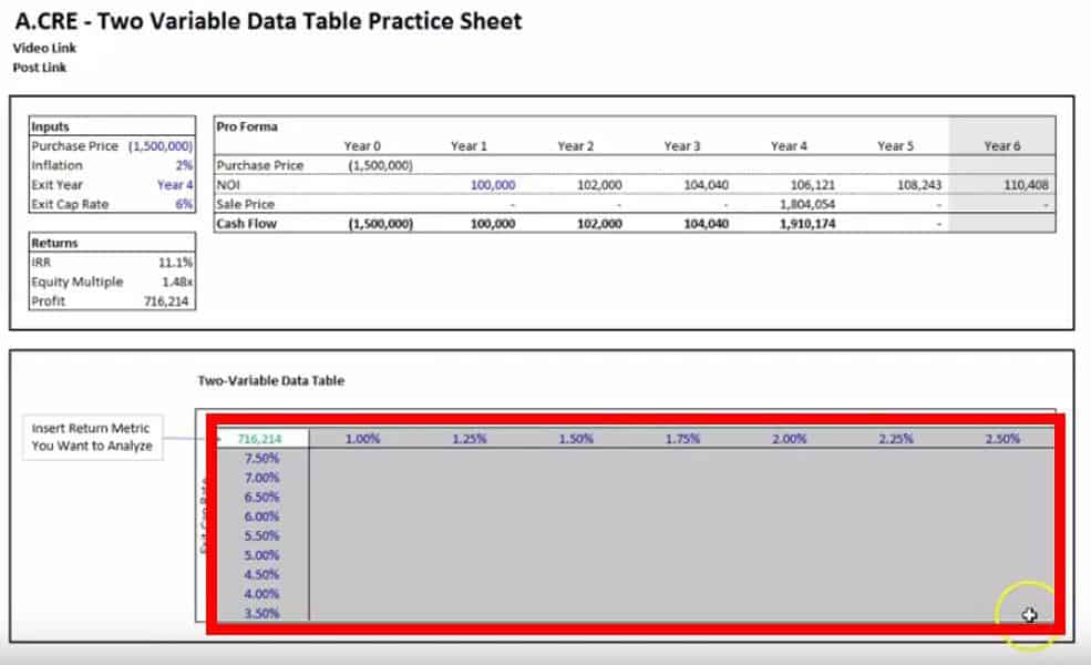
Step 1: Link the Return Metric You Want to Analyze
Find an area on your model where you want to set up the data table and use the top left cell (In the template, this would be cell F23) to link to a return metric. Click the cell and type the equals sign (=) and click the cell with the return metric you want to analyze. In our template this would be either cell D14, D15, or D16.
Step 2: Choose Two Input Assumptions (Variables) and Decide on the Ranges You Would Like to Test
In the template in this post, we have four variables we can choose from: the purchase price, inflation, exit year, and exit cap rate. For this example, let’s pick inflation and the exit cap rate.
Directly to the right of the cell where you linked the return metric you want to test, input any number of potential annual inflation rates you like to analyze. For every new inflation rate you want to test, move one cell to the right and input the new number. If you are working within the template, this area is from cell G23 to M23.
Directly below the cell where you linked the return metric you want to test, input any number of exit cap rates you want to analyze with each new cap rate entered in the cell below (F24 to F32 in the template).
Step 3: Highlight the Area of The Data Table and Open the Data Table Prompt
Highlight the entire rectangle/square of cells that include the linked return metric cell in the top left, the bottom cell that contains the last exit cap rate in the range you input underneath the return metric, and the cell that contains the last inflation number that is the furthest to the right from the return metric. In the template, this area is between cell F23 and M32. See the screen shot from the video below for clarification:
Now, click ‘Data’ at the very top in the green bar > What-if Analysis > Data Table
To do the above without using the mouse type Alt > A > W > T
Step 4: Input the cell references for the column variables and row variables
The final step is to input the cell containing the assumption being tested in the row going across the top in the ‘Row input cell’ (D9 in the template) and to input the cell with the assumption being tested in the column going down the left-hand side in the ‘Column input cell’ (D11 in the template), then click ok and the results should appear in you input table. You may need to format the table if the answers are not displayed in the way you prefer.
Creating Data Tables Part 3: Two Variable Data Tables – How To Display More Than One Return Metric Within a Cell
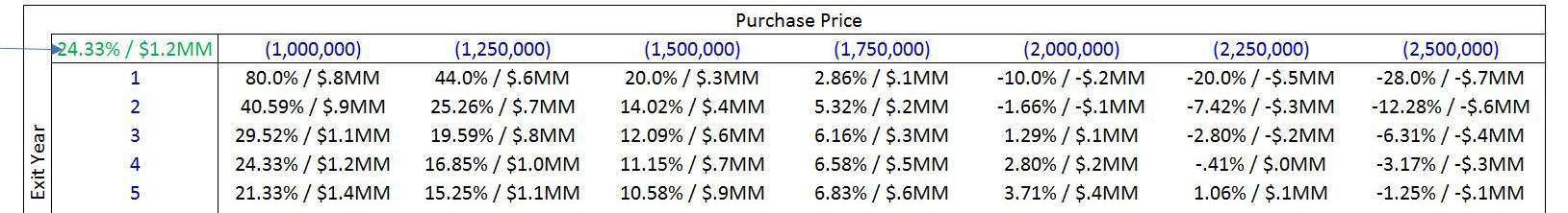
In the third part of this data table series, I’m going to show you how you can create data tables with multiple return metrics within each cell of the data table as shown in the image below.
As with Part 2, there is both a video and a step-by-step guide below;
Video
Step-By-Step Guide
To begin, let’s open the template and click on the cell in the top left of the data table that is the reference cell for the table’s returns. In the template, this is cell F23.
Everything that you need to do in addition to the standard procedure for creating the data table will take place in this cell and you really only need to familiarize yourself with three excel functions.
The Ampersand (&), Quotation Marks, and the =TEXT( ) Formula
Step 1: The Ampersand
The ampersand will allow you to combine and view multiple results from various cells within one cell. However, what it cannot do is format these multiple results in a way that the user can easily read it or in a way that the creator of the data table would want to display the info. For example, let’s combine the profit and IRR into one cell. To do this, type the following formula in cell F23:
=D14&D16
What is returned is the following:
0.2432861997811491216214.4
(Excel Tip: If you can’t see the complete number in the cell, click on cell F23 and type Alt > O > C > A)
If we look closely, you can see both return metrics:
0.243286199781149 1216214.4
The blue is the IRR and the red is the profit.
Step 2: Quotation Marks
The quotation will allow you to add text in between cell references. Using the same formula from above, insert the following:
=D14&” Hello “&D16
(Don’t forget to add the spaces between the quotes and ‘Hello’.)
The result should be:
0.243286199781149 Hello 1216214.4
Now that you see that you can add text between the quotes, erase Hello and in the quotation marks, insert a backslash ( / ), so that the result is:
0.243286199781149 / 1216214.4
Step 3: =Text(value, format_text)
The =Text( ) function will allow you to format the values from the different cells being referenced. =Text is a two part function that asks you to first link the cell you want to reference and then asks you how you want to format the result. In our example, let’s change the current formula from:
=D14&” / “&D16
to this:
=TEXT(D14,”##.#0%”)&” / “&TEXT(D16,”#,###,###”)
The formula should result in this display: 24.33% / 1,216,214
As you can see, we formatted the IRR to show four numbers with a decimal point and a percent sign (“##.#0%”) and we formatted the profit to have commas (“#,###,###”) to display the number properly.
If you would like to display the profit, which is in the millions, in a shorter format, as shown in the image above, you can replace the
“#,###,###”
with
“$#,###.0,,”
and add
&”MM”
onto the end of the formula:
=TEXT(D14,”##.#0%”)&” / “&TEXT(D16,”$#,###.0,,”)&”MM”
Which will give you the following result:
24.33% / $1.2MM
Bonus: Data Tables Not Working? Try This Quick Fix
Download the Source Files for this Watch Me Build Exercise
To make these files accessible to everyone, they are offered on a “Pay What You’re Able” basis with no minimum (enter $0 if you’d like) or maximum (your support helps keep the content coming – similar real estate training exercises sell for $100 – $300+). Just enter a price together with an email address to send the download link to, and then click ‘Continue’. If you have any questions about our “Pay What You’re Able” program or why we offer our models on this basis, please reach out to either Mike or Spencer.
Frequently Asked Questions about Data Tables for Real Estate Sensitivity Analysis in Excel

