Real Estate Acquisitions Model #2 for Office, Retail, Industrial (Updated Apr 2026)
I’ve decided to do a major overhaul of my last acquisitions model for office, industrial, and retail properties. There were a lot of things I wanted to change as well as add to the model and finally had a weekend to do it. This new and improved model includes both monthly and annual cash flows, as well as a returns summary and sensitivity analysis section. All the inputs flow directly to the monthly cash flow section and thus allow for a more precise analysis and ability to dictate when certain cash flows happen on a monthly rather than yearly basis.
For example, there is now the ability to input tax payments and insurance premium payments into a specific month every year growing at X%. Additionally, the IRR is now being calculated using the XIRR excel formula allowing for a much more accurate calculation of this return metric. Below is an overview of the model along with an instructional video. The download is located at the bottom of the post. Feel free to download the model now and continue reading and/or watch the accompanying video.
Are you an Accelerator member? You might review the ‘Building an Acquisitions Model from Scratch‘ course. In that course, we build a single-tenant retail acquisitions model from scratching using the 10000 Fitness Way case study. Not yet an Accelerator member? Consider joining the real estate financial modeling training program used by top real estate companies and elite universities to train the next generation of CRE professionals.

Section 1: Acquisition Inputs
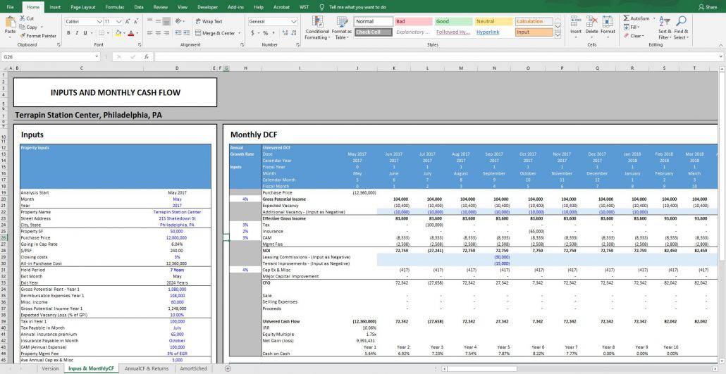
The inputs section is fairly straight forward with a few interesting options. Some of this will most likely be basic for our readers, but nonetheless I will give a brief walk through. As always, the cells with blue text are the true input cells that can be altered while the black cells should be left alone.
Property Inputs – Analysis Start Section
This section has a drop down menu in cell D20 to select the month and in the cell below the user will manually input the year. Setting these inputs will alter cell J13 in the Monthly cash flow portion of the model and the subsequent cells in the ‘Date’ row. This also has an impact on other cells within the input section such as the exit month and year and the inputs that enable the user to select the date in which a one-time large capital improvement can be modeled for.
Property Inputs – Name and Address Section
One thing to note about this section is that the ‘Property Name’ cell and the ‘City, State’ cell will influence the header on all three sheets.
Property Inputs – EGR Inputs
The next section starting in row 34 is where the user will put in first year aggregate annual revenue assumptions. This includes (1) gross potential rent, which is where the user will input all the possible rental income for year one; (2) reimbursable expenses; and (3) miscellaneous income. These three inputs all roll up into Year 1 Gross Potential Income. Cell O38 is where the user will input the expected vacancy loss as a percent of GPI.
Property Inputs – Operating Expenses
Starting in row 39, there are inputs for taxes, insurance, and CAM. With both taxes and insurance, there is the ability to pick the month in which these expenses reoccur every year. Notice that the month payable for both taxes and insurance are July (cell D40) and October (Cell D42), respectively. In the monthly cash flow, you will notice in rows 24 and 25 that these expenses reoccur every year in those months and grow at the annual inflation rate selected in column H.
Property Inputs – Capital Expenditures
Since this model does not go down to the individual tenant level, I decided to make tenant improvements and leasing commissions manual inputs in the monthly cash flow section (rows 29 & 30) and therefore they do not have a dedicated space in the Inputs section of the model.
Cells D46:D51 is where you can input a one-time large capital improvement item and have a percentage of the total cost financed by the loan. This has the same functionality the original model had where the loan will reamortize on the date when the capital improvement occurs, but this time you can choose the month this happens. A cool feature to this function is that the drop down menus in cells D48:d49 will not allow you to choose a funding date that is beyond the exit date.
Property Inputs – Debt Inputs
The debt input section is very straight forward with regard to the inputs. However, one thing to note in this section is the two different loan payments – one before and one after the funding of the capital improvement. When the capital improvement happens, the loan will fund the specified amount asked for, and then reamortize at that date to still have the principle paid off by the time the original amortization schedule specified.
In order to see how this all works, examine the cells in the ‘AmortSched’ sheet and pay particular attention to row C and the box in column L as well as the payment calculation.
Section 2: Monthly Cash Flow
This section should be very straight forward. Note that Row H has the annual growth rate inputs for GPI, tax, insurance, CAM, and cap ex and that rows 22, 29, and 30 are manual inputs for Additional Vacancy, LCs and TIs, respectively.
Section 3: Return Metrics and Sensitivity
On the ‘AnnualCF & Returns’ sheet, we can see the returns summary and sensitivity analysis. In the returns summary, there is an input to allow the user to change the discount rate for the NPV calculations in both the levered and unlevered return summary sections. The sensitivity analysis allows the user to look at both the purchase price and hold period impact on IRR.
Video Walk-through – Real Estate Acquisition Model #2 for Office, Retail, and Industrial Properties
The rest of this model should be fairly easy to interpret and understand. Hope you enjoy it and please feel free to reach out with any questions or comments.
Download the Real Estate Acquisition Model #2 for Office, Retail, and Industrial Properties
To make this model accessible to everyone, it is offered on a “Pay What You’re Able” basis with no minimum (enter $0 if you’d like) or maximum (your support helps keep the content coming – typical real estate Excel modules sell for $100 – $300+ per license). Just enter a price together with an email address to send the download link to, and then click ‘Continue’. If you have any questions about our “Pay What You’re Able” program or why we offer our models on this basis, please reach out to either Mike or Spencer.
We regularly update the model (see version notes). Paid contributors to the model receive a new download link via email each time the model is updated.
Frequently Asked Questions about the Real Estate Acquisitions Model #2 for Office, Retail, and Industrial
Version Notes
v2.4
- Formulas across the Inputs & MonthlyCF, AnnualCF, and Returns tabs have been reviewed
- Placeholder values on all tabs have been refreshed to reflect current defaults.
v2.3
- Added Versions tab
- Updated header on all three worksheets
- Replaced input cells’ soft blue font with true blue font (0,0,255)
- Updated model name
- Misc. formatting enhancements
v1.0
- Initial release


